3. Inferring iModulon activities for new data

Re-computing the complete set of iModulons can be computationally intensive for every new dataset. However, once a dataset reaches a critical size, you can use a pre-computed IcaData object to infer the iModulon activities of a new dataset. iModulon activities are relative measures; every dataset must have a reference condition to which all other samples are compared against.

To compute the new iModulon activities, first load the pre-computed IcaData object.

[1]:

from pymodulon.example_data import load_ecoli_data
ica_data = load_ecoli_data()

Next, load your expression profiles. This should be normalized using whichever read mapping pipeline you use, as Transcripts per Million (TPM) or log-TPM.

[2]:

from pymodulon.example_data import load_example_log_tpm
log_tpm = load_example_log_tpm()
log_tpm.head()

[2]:

	Reference_1	Reference_2	Test_1	Test_2
Geneid
b0001	10.473721	10.271944	10.315476	10.808135
b0002	10.260569	10.368555	10.735874	10.726916
b0003	9.920277	10.044224	10.528432	10.503092
b0004	9.936694	10.010638	9.739519	9.722997
b0005	7.027515	7.237449	6.745798	6.497823

Next, make sure your dataset uses similar gene names as the target IcaData object.

[3]:

from matplotlib_venn import venn2
venn2((set(ica_data.gene_names),set(log_tpm.index)), set_labels=['IcaData genes','Dataset genes'])

[3]:

<matplotlib_venn._common.VennDiagram at 0x7f6f9c174650>

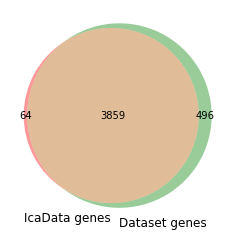
../_images/tutorials_inferring_imodulon_activities_for_new_data_7_1.png

Only genes shared between your IcaData object and the new expression profiles will be used to project your data. All other genes will be ignored.

Then, center your dataset on a reference condition, taking the average of replicates.

[4]:

centered_log_tpm = log_tpm.sub(log_tpm[['Reference_1','Reference_2']].mean(axis=1),axis=0)
centered_log_tpm.head()

[4]:

	Reference_1	Reference_2	Test_1	Test_2
Geneid
b0001	0.100889	-0.100889	-0.057356	0.435303
b0002	-0.053993	0.053993	0.421312	0.412354
b0003	-0.061973	0.061973	0.546181	0.520841
b0004	-0.036972	0.036972	-0.234147	-0.250669
b0005	-0.104967	0.104967	-0.386684	-0.634659

Finally, use the pymodulon.util.infer_activities function to infer the relative iModulon activities of your dataset.

[5]:

from pymodulon.util import infer_activities

[6]:

activities = infer_activities(ica_data,centered_log_tpm)
activities.head()

/home/docs/checkouts/readthedocs.org/user_builds/pymodulon/envs/stable/lib/python3.7/site-packages/pymodulon/util.py:327: FutureWarning: Index.__and__ operating as a set operation is deprecated, in the future this will be a logical operation matching Series.__and__.  Use index.intersection(other) instead
  shared_genes = ica_data.M.index & data.index

[6]:

	Reference_1	Reference_2	Test_1	Test_2
AllR/AraC/FucR	0.243143	-0.243143	1.028044	0.848571
ArcA-1	-0.157687	0.157687	-2.644027	-2.418106
ArcA-2	0.038248	-0.038248	0.182260	0.039267
ArgR	-0.150147	0.150147	-1.456806	-1.293399
AtoC	0.344893	-0.344893	0.632130	1.075412

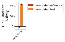
All of the plotting functions in pymodulon.plotting can be used on your inferred activities once you add it to a new IcaData object. It is advisable to create a new sample_table with project and condition columns.

[7]:

from pymodulon.core import IcaData
import pandas as pd

[8]:

new_sample_table = pd.DataFrame([['new_data','reference']]*2+[['new_data','test']]*2,columns=['project','condition'],index=log_tpm.columns)
new_sample_table

[8]:

	project	condition
Reference_1	new_data	reference
Reference_2	new_data	reference
Test_1	new_data	test
Test_2	new_data	test

[9]:

new_data = IcaData(ica_data.M,
                   activities,
                   gene_table = ica_data.gene_table,
                   sample_table = new_sample_table,
                   imodulon_table = ica_data.imodulon_table)

[10]:

from pymodulon.plotting import *

[11]:

plot_activities(new_data,'Fur-1',highlight='new_data')

[11]:

<AxesSubplot:ylabel='Fur-1 iModulon\nActivity'>

../_images/tutorials_inferring_imodulon_activities_for_new_data_19_1.png

[ ]:

[ ]:

[ ]: